
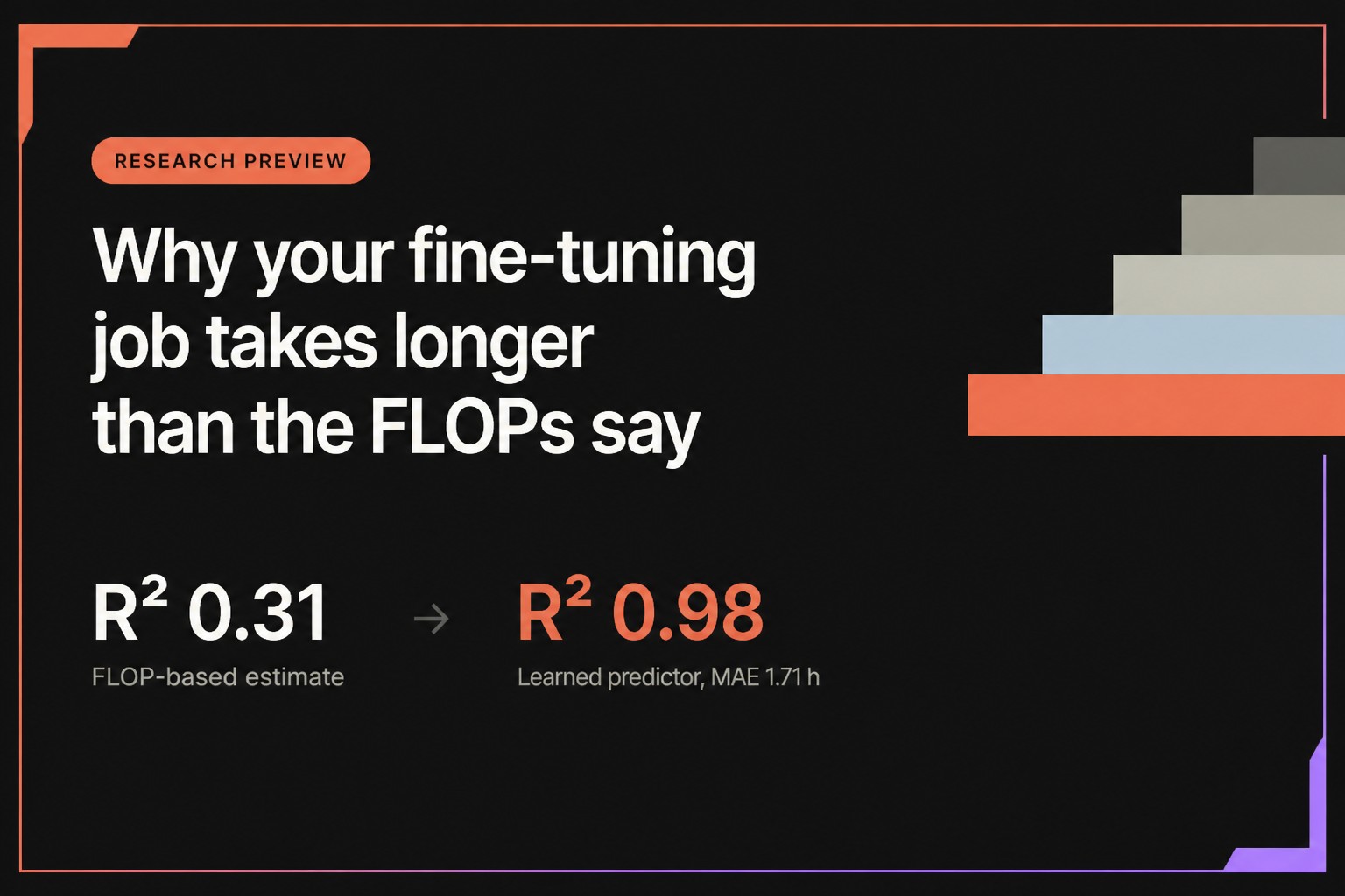
Researchers at Dharma AI compared estimates of fine-tuning time based on operation counts with CatBoost predictions across 272 production runs on NVIDIA H200 GPUs, totaling about 7,382 GPU hours. The conventional estimate explained only a small share of the variation and was off by an average of 12.41 hours. A model using only parameters known before a run achieved R² = 0.98: its mean absolute error was 1.71 hours, and its median absolute error was 0.51 hours. This kind of forecast can help schedule jobs on a shared cluster.
CatBoost predicts fine-tuning time with an error of half an hour
Why computation estimates are not enough
For a dense transformer, training compute is estimated as 6·P·D, where P is the number of parameters and D is the number of training tokens. Dividing this figure by GPU performance gives an estimate of the training cycle time:
T_theoretical = (6 · P · D) / (N_GPU · FLOPS_peak · MFU)N_GPU is the number of GPUs, FLOPS_peak is the peak performance of one device according to its specifications, and MFU (Model FLOPs Utilization) is the share of that performance actually used by training. Jobs do not run at peak performance because of memory transfers, communication between devices, and inefficient compute kernels. MFU is usually between 30% and 60%, but the right value for a specific job cannot be determined in advance.
This formula estimates the optimization cycle, but a full job includes other stages as well. Before training, the environment must be configured, the model loaded and prepared, and tokenization performed. During training, periodic evaluations and checkpoint uploads take place; at the end, the final model is saved to object storage. On a shared cluster, these operations compete with other jobs for network and storage resources.
Overhead depends on configuration and does not scale predictably with job size or the number of GPUs. As a result, two jobs with the same estimated compute can finish hours apart. To make the comparison fair, the authors included evaluation tokens in the baseline FLOP calculation and tested different MFU values.
How the forecast works
The authors treat job duration—from launch on allocated GPUs to completion—as a regression problem. Queue wait time is excluded. All input features come from the configuration submitted before launch: hyperparameters, dataset sizes, model identifiers, and allocated GPUs. Live logs and the model’s intermediate progress are unavailable, which makes this kind of forecast usable for planning.
Alongside the original settings, the researchers calculated features related to overhead: num_eval_data, the number of examples processed across all evaluation cycles; num_saves and num_params_saved, which describe checkpoint operations; and the number of tokens per GPU. The FLOP estimate with a fixed MFU of 0.45 was also included as the baseline_time feature: the model starts with an estimate of compute load, then adjusts it based on other factors.
The authors compared linear regression, Ridge, XGBoost, and CatBoost. They selected features using correlation filtering, mutual information, and permutation importance. They tested 18 feature sets, then ran a grid search, selecting options by mean absolute error. The final CatBoost model included 24 features.
Which jobs were included
The dataset contained 272 supervised fine-tuning (SFT) runs from logs of a corporate production environment. It covered several model families with up to 15 billion parameters, full fine-tuning and LoRA, and datasets and hyperparameters of different sizes.
Jobs ran on one, two, or four GPUs drawn from a shared pool of 8–32 NVIDIA H200s, deployed across one to four nodes. Other training and inference jobs ran on the infrastructure at the same time, so the measurements reflect real competition for resources. Run durations ranged from 1.6 to 172.4 hours, with a mean of 23.43 hours and a median of 15.29 hours.
The software stack included Hugging Face Transformers and Unsloth. The authors treated it as a categorical feature, without assuming in advance that one option would deliver a fixed speed advantage over the other.
Comparing methods
All results came from five-fold stratified cross-validation. The first four baseline methods were analytical and did not require model training.
No MFU value made the FLOP estimate accurate. The authors tested values from 0.25 to 0.65. The best result came with an MFU of 30%, but the mean error still exceeded 12 hours, against an average job duration of about 23 hours.
A more detailed analytical model did not close the gap either. As a second benchmark, the researchers used Calculon, a model for estimating large language model training performance described by Isaev and coauthors at SC ’23. It builds an explicit graph of layers and accounts for computation, memory transfers, and communication between devices. The authors extended the open-source implementation to support LoRA, grouped-query attention, multi-query attention, bfloat16, and SwiGLU. However, its median predicted time was only 11% of the actual duration. The authors say this does not disprove Calculon’s usefulness for estimating individual steps: that was what the model was designed to do. The result shows how much of a production job is spent on operations beyond the optimization step.
Linear models improved the forecast, but their capabilities were limited: Ridge reduced the mean absolute error to 7.23 hours. The relationship between job settings and duration cannot be described accurately enough using a linear relationship alone.
Gradient-boosting methods accounted for most of the improvement. CatBoost and XGBoost differed by no more than one standard deviation across all metrics. The authors selected CatBoost for further analysis because it had the lowest mean error.
Which parameters are associated with duration
CatBoost’s feature importance centers on several parameters, including model and workload characteristics, as well as evaluation and checkpoint settings. The most important was num_eval_data, the total number of examples processed during evaluation across the job. It was followed by num_trainable_params, batch_eval_size_percent, num_all_params, and num_gpus*batch_train_percent; num_params_saved was close behind.
SHAP analysis showed a similar pattern: a larger evaluation workload consistently increased predicted time. The number of trainable parameters had a nonlinear effect, which became noticeable for the largest models. Feature importance alone does not prove causation, but the patterns are consistent with how job time is distributed: the result is affected by the frequency and size of evaluations, the number of checkpoints saved, and the scale of the model and dataset. Many of these parameters are set when the training configuration is prepared.
The number of allocated GPUs is associated with longer predicted times in the model. However, in this dataset, larger allocations also corresponded to larger jobs, so the number of devices partly reflects job scale. This does not mean that adding GPUs, by itself, slows training.
Where accuracy declines
Across all 272 predictions made outside the training folds, the median absolute error was 0.51 hours. The error was no more than 2.20 hours in 80% of cases and no more than 4.31 hours in 90%.
For jobs lasting up to 60 hours, the median error stayed around one hour or less. Predictions became less accurate for longer runs. There were only 13 such jobs, so the authors attribute the decline in performance to a lack of data.
On a fixed held-out set comprising 20% of the data, mean absolute error fell from 1.63 to 1.50 hours as the share of data used for training increased from 85% to 100%. No clear plateau appeared.
Uses and limitations
The forecast lets a scheduler estimate a job’s duration before it starts: which jobs to run concurrently, when GPUs will become available, and whether training will finish by a deadline.
The model was tested only on SFT. Other training strategies and preference-tuning methods, including RLHF, DPO, and RLVR, were not included in the dataset. All runs used H200s, so the numerical results cannot automatically be applied to other GPU generations; the model would need to be retrained. For mixed pools of devices, hardware characteristics would also need to be included: compute performance, memory capacity and bandwidth, and interconnect topology.
The authors say the approach itself can be applied to other infrastructure: features that account for overhead, feature selection that accounts for multicollinearity, and a comparison protocol. The full paper is expected to include feature formulas, the selection procedure, search spaces, and final hyperparameters, making it possible to reproduce the pipeline on a set of execution logs with a similar structure.
Further work could explore hardware-specific features and test the model on other GPU types; transfer learning to configurations with few observations; other training objectives; and collecting more data on long runs. The authors say the full paper will soon appear on arXiv.
Dataist’s take: The results show how much training schedules depend on operations around the compute cycle, particularly evaluation and checkpointing. But the findings so far apply to SFT on NVIDIA H200s; the model’s transferability to other hardware and training setups remains to be tested.
Daily AI news
Every day we pick what actually matters in AI and explain it plainly — no hype, no filler. Subscribe if you want to follow where the industry is going.
Only what matters — every day
Follow on X